Conditional Formatting in Excel based on the contents of another cell

by | Feb 15, 2014

Excel conditional formattingToday I got an interesting question from a customer using Excel for Mac 2011. She wanted to know if she could use Conditional Formatting to color a cell based on the contents of another cell.

In her case, she has notes about employees written in a cell, and wanted to call attention to their salary if there were any notes for that person. To do this,

  1. Click on the first salary cell that you would color if the row has a note.
  2. Click on Conditional Formatting.
  3. Choose New Rule.
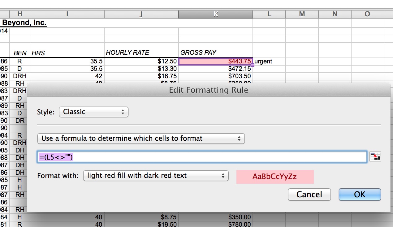
  4. Drop down the Style option and change it to Classic.
  5. Drop down the next option and select Use a formula to determine which cells to format.
  6. Enter the formula as =(N3<>””), with N3 being the first cell with a potential memo in it. This tells Excel to use the formatting if the cell does not equal null (is not empty).
  7. Edit the formatting to your liking (text color, fill color).
  8. Close the dialog box.
  9. Click back on the cell.
  10. Use the AutoFill Handle (the little square in the bottom right corner of the cell outline) to replicate the cell down the entire column.
  11. Any of the cells that have notes will now turn colors.

Using Conditional Formatting to automatically highlight cells based on criteria is a powerful way to create dynamic spreadsheets!

Udemy Course Learn Excel in 3 Hours Flat


Need to learn Excel quickly? Check out Alicia’s online course, Learn Excel in 3 Hours Flat. For only $59 you get lifetime access to the course.


About Alicia Katz Pollock

With a Masters in Teaching from Tufts University, a QuickBooks®️ Online Advanced Certification and more than 30 years’ experience in the tech industry, Alicia is passionate about finding creative, practical solutions to complex and everyday tech problems. She also loves a good laugh!

Comments

9 Comments

  1. Celeste

    I am trying to format the cells in the classic style formating the cells using a formula. The format I am using is =$A$2=”N” format with: light red fill with dark red text. Is there a way I can copy and paste my formula on each row in the spreadsheet without having to change the selected cell each time? I have tried ctrl + D and it does not work.

    Reply
  2. Saul

    Hello and thank you for your tip.
    I’m using Excel 2019 for Mac and wondering if you can help me.
    Here you are talking about coloring a cell based on a different cell’s value.
    I would like to do the same, but instead of a single character/value as the criteria, a character or value within a string.
    IE, to color A2 if A1 contains the word “example” (when A1 contains a phrase like “For example, 4×4”).
    I have some ideas but none of them worked so far. :-))))
    Thanks in advance
    Saul

    Reply
    • Alicia Katz Pollock

      Hi Saul, Yes, you can! In Conditional Formatting, go down to the bottom to create a New Rule. Make the Style “Classic.” Choose Format Only Cells That Contain, then Specific Text, then Containing. type in your string! That should do it.

      Reply
  3. Vidya

    Can I set a value of a cell based on text value of another cell with the same background color?

    Reply
    • Alicia Katz Pollock

      If you google it, I saw someone combine an IF statement with a Macro that assigns numerical values to cell fills. But there’s no native functions to do that.

      Reply
  4. Gert

    If I wanted to edit a bank statement and color the amounts according to whether they are credit or debet (which is the next column). How could I do that?
    Dragging the Autofill on the first amount left me with a column of the same amounts…

    Reply
    • Alicia Katz Pollock

      When you use the Autofill Handle, it will overwrite the content BUT immediately click on the little Smarttag that appears. It will have an option to “Copy Formatting Only”. When you click on it, you’ll get your numbers back, and just get the Conditional Formatting to change the colors.

      Reply
  5. Alicia Katz Pollock

    Use the standard logical formulas and nest the conditions inside: =and(I5>35,L5<>“”)

    (Hours are greater than 35 and there’s something in L5).

    Reply
  6. Aditya

    In case we wish to apply multiple conditions, then how does one use logical operators like “or”, “and” and “Not” ?

    Reply

Submit a Comment

Your email address will not be published. Required fields are marked *